10+ Google Sheets Functions and Formulas for Mastering Keyword Mapping

I can’t help but wonder sometimes how many techniques SEO has. One of them is keyword mapping, a process of researching and assigning keywords to different pages you work with. It is a crucial and insightful part of planning and developing a website.

There is, however, a hurdle: keyword mapping requires a lot of manual, often tedious labor. But given how valuable the outcome is, SEO professionals definitely shouldn’t bypass this technique.

Here is the good news: we can make keyword mapping easier, faster, and more efficient using the spreadsheet software. The two most popular solutions are MS Excel and Google Sheets. I am a big fan of the latter, so in this article, I will tell you how to ace keyword mapping with Google Sheets by utilizing several functions and combining them in powerful custom formulas.

Preparations and Data Export for Keyword Mapping

I will use Ahrefs as a source of keyword data. The first step we need to take is to add the project. For the article, I will use my favorite website “Analytics Mania” founded by a great web analyst and creator Julius Fedorovicius.

After the project is added, proceed to the project page, where you will find lots of different reports on the website. First, familiarize yourself with the “Site structure” report, to recognize categories there are, because this kind of information is a must for keyword mapping.

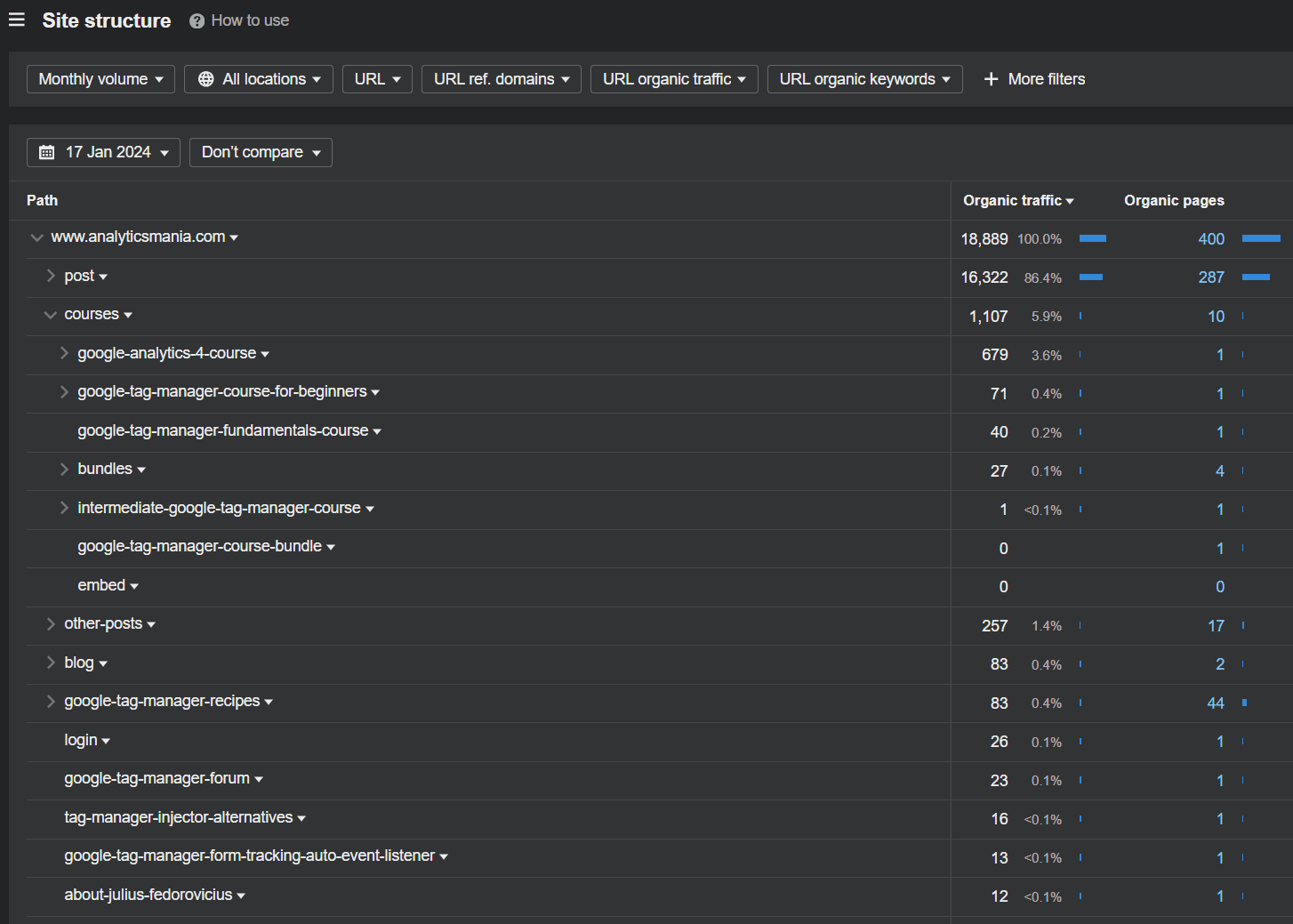
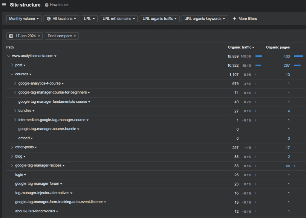
So, “Analytics Mania” has a few URL folders: “post” (slug is /post/), “courses” (/courses/), “other posts” (/other-posts/), “GTM recipes” (/google-tag-manager-recipes/), and a handful of standalone pages.

Next, it is the turn of keywords. On the project’s page, navigate to the “Organic keywords” report. It shows keywords by country, and by default, you will see the country with the biggest number of keywords a website ranks for. In the case of “Analytics Mania”, it’s the USA (~12,700 terms). I pick a smaller list of keywords from the UK (about 2,200 keywords).

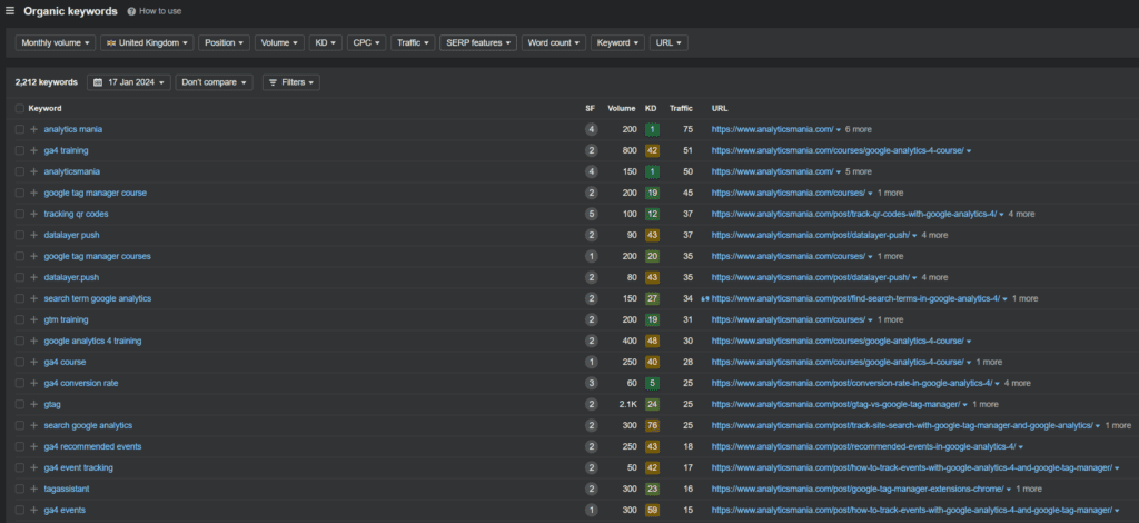
A remark: hypothetically, we could also use the “Top pages” report, but it only shows one query that brings in the most traffic per page, which does not work for our case. There is also an option of examining each ranking page separately, but I honestly don’t find it convenient. The best solution is to gather all the data we need in one spreadsheet.

I download the file, then upload it to Google Sheets, and open the sheet.

The exported file has keywords, and the rows contain some data on each keyword, such as position and search volume, and also a page URL that ranks for this keyword in the far right column:

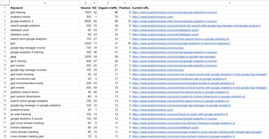
All the keywords in the “Keyword” column are unique, but the “Current URL” column contains a lot of duplicates because one page may rank for various keywords. We want to get the opposite spreadsheet, where data will be arranged by web pages, not keywords.

Duplicate the list to keep the original one intact. I did not think much and called the new list “Duplicate”.

Our first step will be to check data integrity.

Step 1: Finding Empty Cells with COUNTBLANK

We need to make sure the data is clean, in particular, that there are no empty cells. I will do it with the simple function called COUNTBLANK, which finds blank cells in the range you specify inside the brackets.

Write the function down in the row next to the bottom end of the spreadsheet. Here is how the formula looks for the column A in my sheet:

=COUNTBLANK(A2:A2213)

The function returns zero, which means there is no missing data.

Step 2: Selecting Unique Values in Google Sheets

Next, we need to retrieve a list of distinct URLs from the “Current URL” column and arrange it vertically. I create a new blank list called “Pages”, and enter the following formula in its A1 cell:

=UNIQUE(ArrayFormula(Duplicate!D:D))

This formula copies the selected column (D) but only with unique values. I will break it down into parts:

• Duplicate!D:D contains the range (column D, where URLs are), and the reference to the list (Duplicate) where this column is located, separated by a special symbol (!).
• ArrayFormula function allows us to perform multiple calculations on one or more items in an array. It can process a range of cells, performing calculations row by row or cell by cell.
• Finally, the UNIQUE function returns a list that includes only one instance of each distinct value found within the given range, removing any duplicates.

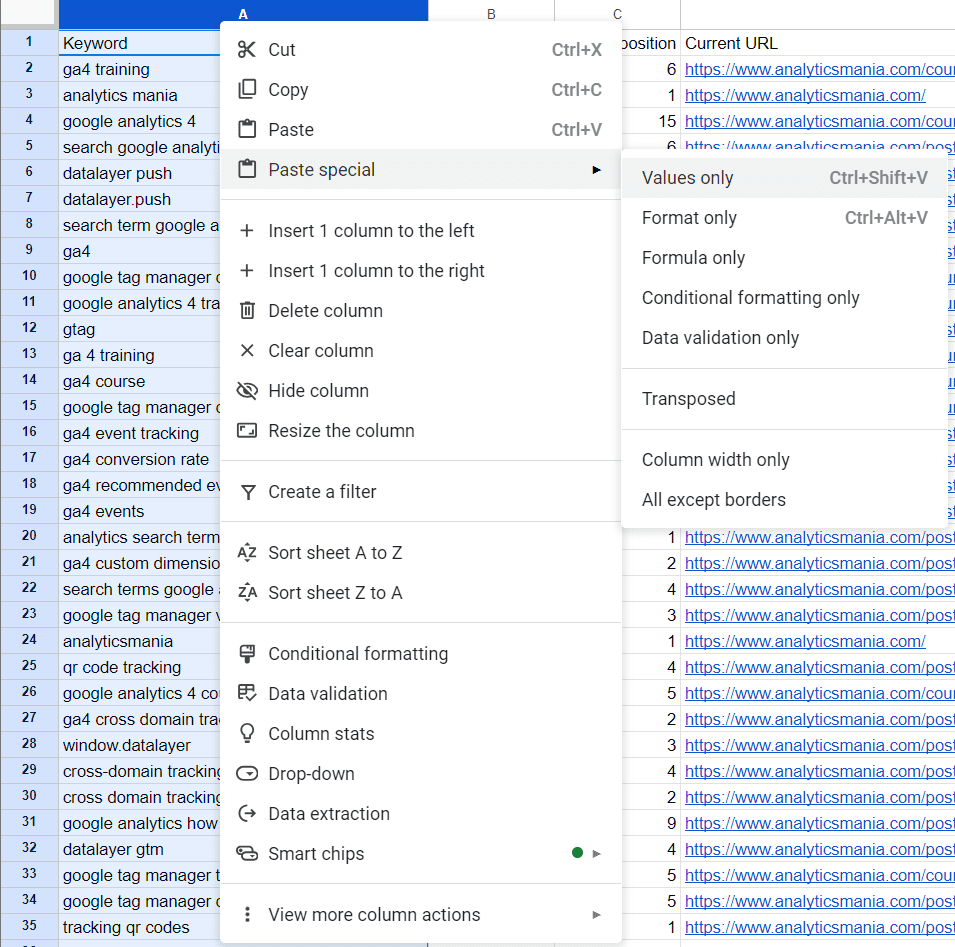
Do not forget to clean the column of the formula so you can manipulate those values. The easiest way to do that is to:

1. Select the entire column by clicking its letter.
2. Right-click on it, and select “Copy.”
3. Then hover on the “Paste Special” option from the drop-down menu.
4. Finally, click on “Values only”.

Check the screenshot for more details:

Step 3: Importing Keywords to a New Google Sheets List Using JOIN and FILTER

The next step is to fetch keywords for each page and arrange them by corresponding URLs in our new “Pages” list, so we could see what keywords our pages rank for.

I write a title “Keywords” for column B, and add the following formula in cell B2:

=JOIN(",", FILTER(Duplicate!A2:A, Duplicate!D2:D=Pages!A2))

As a result, we get a list of keywords in column B for each URL, put in one cell and separated by a comma (it looks like a mess, but we will work that out a little bit later):

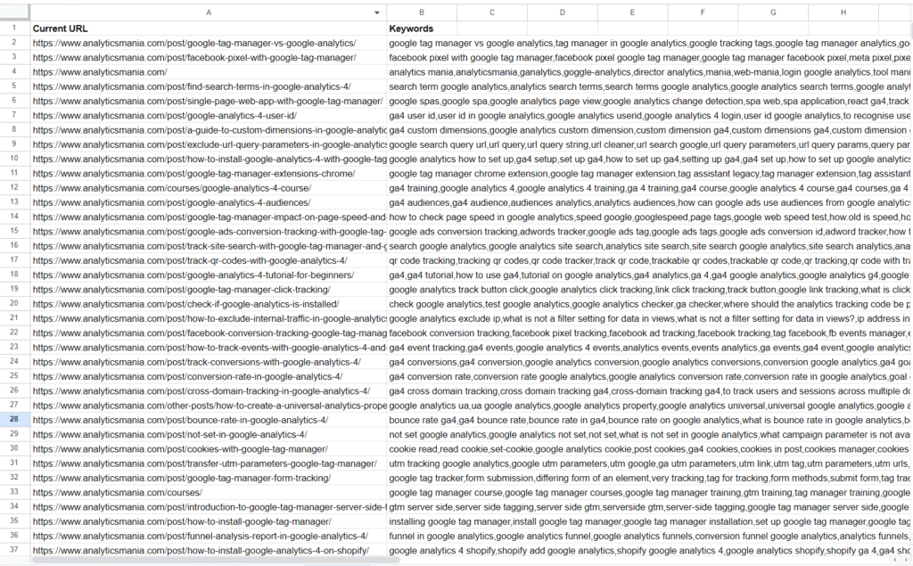
Here is the explanation of this formula:

• The FILTER function returns a range that meets certain criteria. In our case, the range is A2:A in the “Duplicate” list, and the condition Duplicate!D2:D=Pages!A2 checks every keyword from column A so its URL value in column D matches the URL value in column A of the “Pages” list (where we export keywords to).
• The JOIN function is needed to concatenate (combine) all the values returned by the FILTER function into a single string, putting all values in one cell. The first argument inside quotes is the delimiter, which is a comma. If you try it yourself, make sure you don’t leave spaces, otherwise you might face problems with processing these cells. 

To be able to manipulate the new “Keywords” column, do not forget to get rid of the formula by copy-pasting cells with the method described in the previous paragraph.

Step 4: SPLIT and COUNTA Functions to Count Multiple Keywords in One Cell

Now, we should start analyzing data. One simple way of doing that is to calculate the number of keywords for each URL, which will help us to compare their SEO performance.

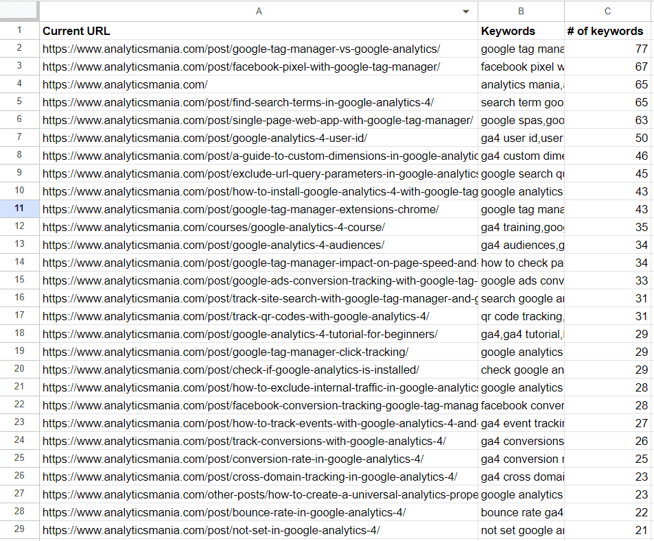
I put a title “# of keywords” to column C in the list “Pages” where we work, and write down the following formula in the first cell, C2:

=COUNTA(SPLIT($B2, ","))

It consists of two parts:

• The SPLIT function separates keywords that are written in a certain cell of each row in the “Keywords” column B based on the indicated delimiter (comma).
• To count the number of separated keywords in each cell, I apply the COUNTA function.

Anyway, you can observe the outcome in the screenshot:

After we get the number of keywords for each page, it makes sense to sort the list by the keyword count. For that, we can apply the built-in function “Sort sheet from Z to A”, which is found by right-clicking on the column C letter. It will give us an understanding of how each page performs, and which ones lag behind our expectations.

To perform the sorting successfully for all columns, check that none of them has the formula left, replace it with the “Values only” method if needed.

Step 5: VLOOKUP and FLATTEN for Studying Separate Pages

Next, we can look at the pages for a certain website category to identify their current state and use keywords for future work. I will make the example of the “Courses” category.

First, I create (again!) a new list where we will transfer the data on these category pages. We need to find pages from this category.

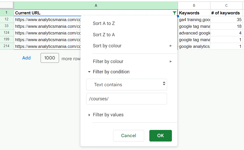
To do this, I return to the “Pages” list, then right-click the column A letter, and select the option “Create filter” from the drop-down menu.

Next, I push the filter sign in the upper column cell, and choose the option “Filter by condition”. Then, select the option “Text contains”, and enter the category slug (/courses/) in the text field. With these simple steps, we get the slice of the sheet that we need:

Just copy-paste all the values to the new sheet we created using the same “Values only” method.

We can continue looking at the pages by turning our new list into a real dashboard. Specifically, I will make a separate “mini-sheet” for every link we imported.

To do this, I write the slug of the first page in a neighboring cell D1, which will serve as the title. Then, I merge it with the cell F1. Below, in cell D2, I put a name for the column, “URL’s keywords”. Then, I extract keywords for this specific page to cell E3 using another formula:

=FLATTEN(SPLIT(B2, ","))

Here are its elements: 

• We have already used the SPLIT function in this project, it divides the given cell value based on some delimiter, and in this case, it is a comma.
• The FLATTEN function organizes these values vertically.

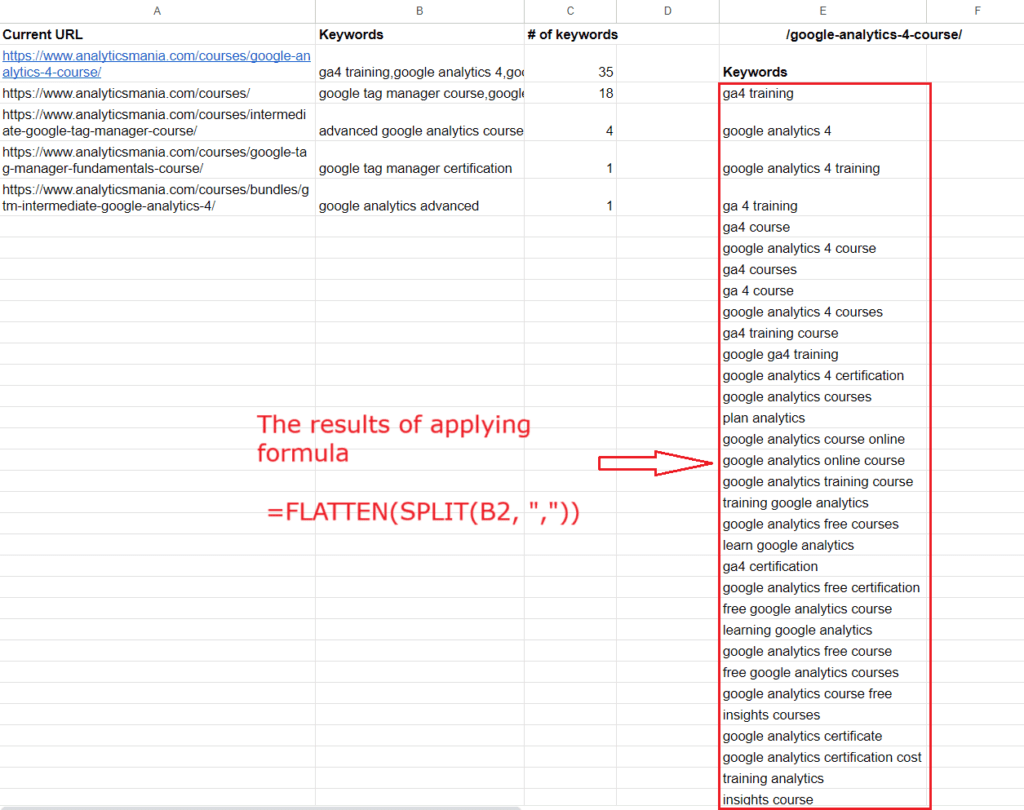
The same can be done with other links.

Remember how we exported data on search volume for each keyword from Ahrefs? We can add this data to the mini-table on our pages, utilizing the legendary Vertical Lookup (VLOOKUP) function.

I start with creating a column next to the “URL keywords”, then enter the formula in cell F3:

=VLOOKUP(E3, Duplicate!A2:B2213, 2, false)

Data is exported successfully, and the results can be seen on the screenshot:

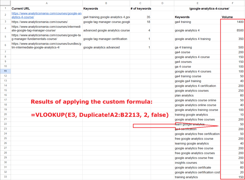
The VLOOKUP function is not as complex as it seems, but might be confusing. It consists of 4 arguments:

1. The first argument is the lookup value, which the function will look for. In this case, I use the keyword “ga4 training” in cell E3 as the key.
2. The part Duplicate!A2:B2213 specifies the range to search for the lookup value. The argument refers to the list named “Duplicate”, and the range always includes the column with the keys from the first argument.
3. The third argument contains the digit “2”, specifying the order number (starting from the left) of the index column where the return value (the one we want to find, the “Volume”) is located. Since the range is from A to B (two columns), 2 means the function will return a value from the second column of this range, which is column B.
4. Finally, the fourth argument is written as either true or false (quoted). It determines whether to look for the exact match (“false”), or the approximate match (“true”). The “false” is considered the default input by Google.    

Using VLOOKUP, you can import other keyword parameters from the original sheet exported from Ahrefs, such as Position, Keyword Difficulty, and so on.

Further Steps

With formulas from this article, the process of keyword mapping for your website becomes much easier. After you finish with the “decomposition” stage, try identifying pages in need of search optimization.

For instance, you can select pages with only a few ranking keywords in each category, or with low positions for certain keywords. For instance, keywords where your URLs are on positions 11-30 present a great opportunity to improve page rankings. Another low-hanging fruit for SEO would be keywords with high potential, i.e. having a decent search volume but low difficulty. Optimizing existing pages, and posting new ones is a good improvement plan.

Conclusion

In this article, I show that basic data analysis can give you much more flexibility and convenience when studying raw SEO-related data within the keyword mapping, than using the limited functionality of even such a powerful SEO tool like Ahrefs. Google Sheets can bring you new ways of discovering helpful insights. Just remember to employ creativity as there is no single line of work in SEO, and every case is individual. Good luck to you on your professional journey!